Three backends, one decision
Jaeger, Zipkin, and Grafana Tempo answer the same question — where do the spans go — with three different bargains. Jaeger is the full platform: one binary as collector, query, and ingester, backed by a database you operate. Zipkin is the oldest and simplest: four components, one Java jar, storage built on Cassandra. Tempo is the newest shape: a backend that needs only object storage and answers with TraceQL.
What each backend actually is
Jaeger v2 ships as a single binary that runs as all-in-one, collector, query, or ingester. The container run exposes port 16686 for the UI, 4317 and 4318 for OTLP, and 9411, with a YAML file passed through the --config flag. Collector and query are stateless. Service maps need the spark-dependencies job.
Zipkin has four components: collector, storage, search, and web UI. Spans arrive by HTTP, Kafka, or Scribe, and are queried through a JSON API. The quickstart is one jar — java -jar zipkin.jar, JRE 17 or newer — at localhost:9411/zipkin. There is no built-in authentication in the UI, so an exposed Zipkin server needs a proxy or firewall in front of it.
Tempo is the outlier. Its own overview says it is cost-efficient and only requires an object storage to operate; its configuration reference lists Amazon S3, GCS, Azure, and the local filesystem, with Memcached or Redis to speed up queries. Tempo accepts Jaeger, Zipkin, and OpenTelemetry protocols, so an existing instrumented fleet can point at it without re-instrumenting.
Storage backends and retention
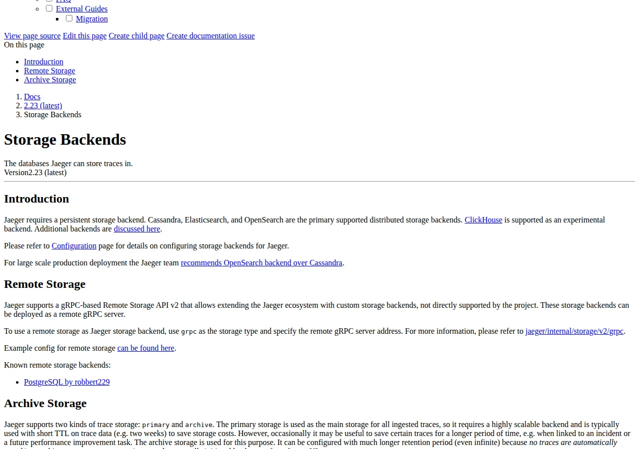
Jaeger requires a persistent backend: Cassandra, Elasticsearch, and OpenSearch are the primary backends; ClickHouse is experimental. For large-scale production the Jaeger team recommends OpenSearch over Cassandra. Jaeger splits storage into primary and archive: the primary store is typically run with a short TTL, for example two weeks, while the archive holds only traces a user saves manually from the UI.
Zipkin’s storage story is narrower and older. It was built on Cassandra, and natively supports Elasticsearch and MySQL. Cassandra needs 3.11.3 or newer; Elasticsearch is tested against versions 7 to 8 and OpenSearch 2. MySQL is a legacy v1 component with known performance issues — queries will eventually take seconds once the volume grows. Dependency links need the zipkin-dependencies Spark job; switching search off leaves traces retrievable by ID only.
Tempo’s storage model is a single formula from its own configuration documentation: ingested bytes per day times retention days equals stored bytes. Its default block retention is 336 hours — 14 days — set by the block_retention option, and blocks are capped at 100 GiB by default. That is why Tempo’s bill is lower: stateless compute plus a bucket.
| Dimension | Jaeger | Zipkin | Tempo |
|---|---|---|---|
| Storage | Cassandra, Elasticsearch, OpenSearch | Cassandra, Elasticsearch, MySQL (legacy) | S3, GCS, Azure, local filesystem |
| Retention | Short TTL (e.g. two weeks) | Limited TTL; QUERY_LOOKBACK 24h | 336h (14 days) |
| Authority | jaegertracing.io/docs/2.23/storage | zipkin.io architecture; openzipkin README | grafana.com/docs/tempo/configuration |
Sampling: the dial that sets the bill
Sampling decides the monthly cost: every span that survives must be stored and retained. Head-based sampling decides at the start of the trace, in the OpenTelemetry SDKs. Tail-based sampling decides after the trace completes, so it can keep every error trace — but the application must export all traces, and the backend pays higher memory and processing costs. Remote sampling centralises the policy: probabilistic at 0.1 keeps about 1 in 10 traces; rate limiting at 2.0 keeps 2 per second.
Zipkin’s sampling is one knob: COLLECTOR_SAMPLE_RATE, the percentage of traces to retain, defaulting to 1.0 — keep everything. It is a head-based decision at ingest, and the server has no tail-based stage. Tempo has no sampling knob of its own: the decision is made upstream, in the SDK or the Collector, and Tempo stores what arrives.
The table below prices sampling at 100 million produced spans a month, at the 1 KB per span assumption stated in the next section, on Grafana Cloud Pro.
| Sampling rate | Spans stored per month | GB ingested | Grafana Cloud Pro monthly cost |
|---|---|---|---|
| 100% | 100,000,000 | 100 | $44.00 |
| 10% | 10,000,000 | 10 | $19.50 |
| 1% | 1,000,000 | 1 | $19.05 |
| 0.1% (Jaeger default) | 100,000 | 0.1 | $19.01 |
Query cost: finding the trace is the second bill
Finding the trace is the second bill. Tempo’s answer is TraceQL, a query language modelled on PromQL and LogQL that selects traces by span attributes. TraceQL requires Parquet, Tempo’s default block format, and TraceQL metrics can generate metrics for alerting. There is no separate index to pay for.
Jaeger’s query path is the UI and API on port 16686, with Service Performance Monitoring for rate, errors, and duration. Zipkin’s query is simpler: find traces by service, operation, tags, and duration, or jump to one from a log-file trace ID. The dependency diagram needs the zipkin-dependencies Spark job. Switching search off cuts storage and write load, but the UI then only opens traces by ID.
What Grafana Cloud Traces costs
Grafana Cloud Traces is Tempo as a managed service, priced in three parts. The free tier is $0 with 50 GB a month and 14-day retention. Pro carries a $19 monthly platform fee including 50 GB a month, with 30-day retention. Usage rates are $0.05 per GB to process, $0.40 to write, and $0.10 to retain. Enterprise is custom, with a $25,000-a-year minimum commitment. The page’s FAQ defines the three lines: process receives and optimises signals; write stores only useful data; retain protects stored data.
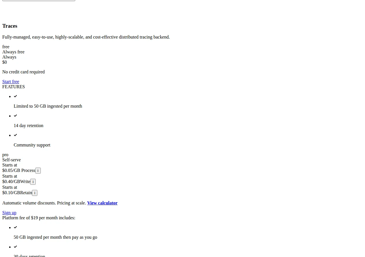
First, this article charges process at $0.05 on every ingested gigabyte and write at $0.40 only above 50 GB; if an invoice waives process inside the 50 GB, subtract $0.05 times the smaller of volume and 50. Second, the retain line prices retention beyond the included 30 days, so the primary model uses the default 30-day retention at $0.45 per GB all in, and shows $0.55 per GB as the upper bound.
One span is modelled as 1 KB of stored trace data — a stated assumption. Real spans vary, so measure your own export. At that conversion, 10 million spans is 10 GB, 100 million is 100 GB, and 1 billion is 1,000 GB a month.
| Spans per month | GB ingested | Grafana Cloud Free | Grafana Cloud Pro | Pro, upper bound with retain |
|---|---|---|---|---|
| 10,000,000 | 10 | $0 | $19.50 | $20.50 |
| 100,000,000 | 100 | Over the 50 GB limit | $44.00 | $54.00 |
| 1,000,000,000 | 1,000 | Over the 50 GB limit | $449.00 | $549.00 |
The self-hosted math
Self-hosted cost is compute plus storage. Compute is one stated assumption: a 4 vCPU, 8 GB server at $40 a month. Storage is priced from a vendor page opened this cycle: Hetzner Object Storage charges €6.49 a month, including 1 TB of storage and egress; over-quota storage is €0.0087 per TB-hour — €6.47 per TB-month. At a stated €1 = $1.16, the base is about $7.53 a month.
Tempo’s self-hosted total is the compute server plus the object-storage base, because Tempo needs only object storage:
That total holds at all three volumes: stored bytes stay under the included 1 TB until about 2,143 GB ingested a month. Jaeger and Zipkin cost more: the database is a second server, $40 for the backend plus $40 for the database node, or $80 a month before the database disk — the database is the cost that scales, not the backend.
Retention is where the self-hosted bill moves. Extending Tempo from 14 days to 90 days at 1,000 GB ingested a month stores 3,000 GB against the 1 TB included, so two extra terabytes at €6.47 each add €12.94, taking storage to €19.44, about $22.55, and the monthly total to $62.55.
The breakeven is where the managed formula meets $47.53: about 108 GB ingested a month on the primary model, about 88 GB on the upper-bound model. Below that band, Grafana Cloud is cheaper — and below 50 GB a month the free tier is $0. Above it, self-hosted Tempo wins: at 1 billion spans the managed bill is $449.00 against $47.53 self-hosted, a 9.4-times difference.
The decision
| Dimension | Jaeger | Zipkin | Tempo / Grafana Cloud | Authority |
|---|---|---|---|---|
| Monthly cost | $80 + disk | $80 + disk | $44.00 / $449.00 managed; $47.53 self-hosted | Grafana; Hetzner pricing |
| Storage | Cassandra, Elasticsearch, OpenSearch | Cassandra, Elasticsearch, MySQL | S3, GCS, Azure; no database | Cited docs |
| Retention | Short TTL, e.g. two weeks, plus archive | Limited TTL; 24h lookback | 336h (14 days) | Jaeger; Zipkin; Tempo docs |
| Sampling | Head, tail, remote, adaptive | Sample rate, 1.0 default, head-based | Decided upstream in SDK/Collector | Jaeger; Zipkin docs |
| Query | UI + API; SPM needs store | UI + JSON API; dependency job needed | TraceQL on Parquet | Cited docs |
Who should not pick each one
Do not pick Jaeger without a database operator: every span lands in Cassandra, Elasticsearch, or OpenSearch, so the team adopts two systems, not one. Do not pick Zipkin for large volumes or long retention: MySQL is legacy, and the default sample rate of 1.0 keeps everything. Do not pick Tempo self-hosted if nobody owns the bucket, the retention, and the upgrades — a 14-day default still deletes last month’s incident traces. Do not pick Grafana Cloud above roughly 100 million spans a month if the team already operates infrastructure: there the managed bill is nine times the self-hosted bill.
Run the switch
- Measure the span size: export one day of spans; divide bytes by span count.
- Set the sampling policy: pick the rate per service — 100% for payments, 1% for health checks.
- Size the retention first: decide the incident window — 14, 30, or 90 days.
- Stand up the backend beside the current one: run the new backend in parallel for one incident cycle.
- Point the collectors: change the exporter endpoint in the Collector or agent configuration.
- Verify the query path: run the three queries the team uses and confirm each answers.
- Confirm the retention clock: check old blocks are deleted on schedule.
- Cut over and watch the bill: compare the first bill against the model and record the variance.
- [x] Real span size measured; 1 KB assumption replaced.
- [x] Sampling policy recorded per service.
- [x] Retention window decided; stored bytes computed.
- [x] Three real queries verified before cutover.
- [x] Retention deletion confirmed; archive holds incident traces.
- [x] First bill compared against the model; variance recorded.
Failure modes
Most tracing migrations fail on the meter. The 100% default: a Zipkin deploy left at COLLECTOR_SAMPLE_RATE 1.0 stores every span until the disk fills. The tail-sampling trap: a Jaeger team enables tail sampling without sizing memory — the application must record and export all traces first. The retention surprise: a team needing 90 days discovers Tempo’s 14-day default only after the traces are gone. The index bill: a Jaeger team on Elasticsearch that never configures rollover or ILM watches daily indices pile up. Each is preventable by setting sampling, retention, and authentication before the first production span.
Founder & CEO Insight — Enow A. Jovial
Measure, sample, size retention, run in parallel, verify queries, then cut over. The pipeline behind these backends is our OpenTelemetry Collector versus Datadog Agent versus Grafana Alloy guide; the managed trio: our Datadog versus Grafana Cloud versus New Relic guide; the error-tracking comparison: our Sentry versus Grafana versus Honeycomb guide. Before the next renewal, run the numbers through our pricing calculator to confirm the volume sits on the right side of the breakeven.