Every factory carries costs that refuse to sit still on one product. Rent, machine depreciation, the supervisor's pay, the power that runs the line — none belongs to a single unit, yet each unit sold must carry its share. Cost allocation gives each unit that share, and overhead absorption moves the cost from the factory floor into inventory and, at sale, into cost of goods sold. Get it right and product costs tell the truth. Get it wrong and the price list rewards the products that lose money and punishes the ones that earn it.
This playbook covers the operation itself: the predetermined overhead rate, the choice of allocation base, plantwide rates against activity-based costing, and the month-end reckoning when actual overhead misses the estimate. The absorbed cost lands in inventory and moves to cost of goods sold when units sell; how that inventory is then valued under FIFO, LIFO, or weighted average is a separate choice, covered in inventory valuation.
What manufacturing overhead actually is
Manufacturing overhead is every factory cost that is not direct materials and not direct labor. Direct materials can be traced to a unit: the steel in the part, the fabric in the shirt. Direct labor can be traced too: the hours the operator spent on that job. Overhead is the rest of the factory — indirect materials such as lubricants and cutting fluid, indirect labor such as supervisors and maintenance crews, factory rent, factory utilities, equipment depreciation, and factory insurance.
Two boundaries keep the pool honest. First, only factory costs enter it. Selling costs and general office costs stay out; the sales team's pay and the head office lease are period costs, expensed when incurred, and they never ride into inventory. Second, abnormal costs stay out as well. Under ASC 330, abnormal freight, handling, and spoilage, plus idle-capacity cost beyond normal levels, are current-period charges. Normal spoilage can be absorbed; a fire in the warehouse cannot be spread across good units to hide it.
The pool is a budget built from the factory's own records: last year's actual overhead, adjusted for known changes such as a rent rise, a new machine, or a planned shutdown.
The predetermined overhead rate
Overhead cannot wait until year end. Jobs need a cost while they are still on the floor, and the books need inventory values at each month end. The answer is a rate set before the period starts, from estimated overhead and an estimated base:
Take a shop that expects $480,000 of manufacturing overhead for the year and 24,000 machine hours of work. The rate is $480,000 divided by 24,000, which is $20 per machine hour. A job that runs 1,200 machine hours absorbs $20 times 1,200, which is $24,000 of overhead. The applied amount is charged to work in process as the job runs:
The estimate is the whole game. Set the base too high and the rate comes out too low, so every job absorbs too little. Set it too low and jobs carry cost the factory never spent. The most common failure is the base, not the arithmetic: a shop that budgets 24,000 hours and runs 20,000 has set its rate on a year that never happened.
Picking an allocation base
The base is the bridge between the overhead pool and the product. A sound base moves with the cost it carries: if machine time drives power, depreciation, and maintenance, machine hours should carry the pool. If hand work drives the cost, direct labor hours should carry it. The table below compares the usual bases and names the authority for each treatment.
| Allocation base | Best fit | Risk if misused | Authority |
|---|---|---|---|
| Direct labor hours | Labor-heavy assembly | Overstates cost where machines do the work | ASC 330-10-30; CFI ABC guide |
| Machine hours | Machine-paced lines | Understates cost of hand-finished goods | ASC 330-10-30; CFI ABC guide |
| Direct labor cost | Shops where pay tracks skill | Breaks when wage rates differ by shift | ASC 330-10-30 |
| Units produced | Single-product plants | Hides every difference between products | ASC 330-10-30 |
One base cannot fit a mixed factory, which is why activity-based costing exists — the worked example below shows the error in dollars.
Worked example: one plant, two products, two answers
A plant makes two products and carries $480,000 of manufacturing overhead for the year. Alpha is simple and high volume: 10,000 units, 20,000 direct labor hours, 2 hours per unit. Beta is complex and low volume: 1,000 units, 4,000 direct labor hours, 4 hours per unit. Direct cost per unit is $55 for Alpha (materials $30 plus labor $25) and $110 for Beta (materials $60 plus labor $50).
Under one plantwide rate, the base is 24,000 direct labor hours and the rate is $480,000 divided by 24,000, which is $20 per direct labor hour. Alpha absorbs 2 hours times $20, which is $40 per unit, for a unit cost of $55 plus $40, which is $95. Beta absorbs 4 hours times $20, which is $80 per unit, for a unit cost of $110 plus $80, which is $190. Applied totals check: $400,000 plus $80,000 is $480,000.
Now split the same $480,000 into two activity pools. Pool one is machine operations at $300,000, driven by 20,000 machine hours: Alpha uses 8,000 hours and Beta uses 12,000. The rate is $300,000 divided by 20,000, which is $15 per machine hour. Pool two is setups at $180,000, driven by 180 setups: Alpha needs 20 and Beta needs 160. The rate is $180,000 divided by 180, which is $1,000 per setup. Alpha absorbs 8,000 hours times $15 plus 20 setups times $1,000, which is $120,000 plus $20,000, which is $140,000, or $14 per unit. Beta absorbs 12,000 hours times $15 plus 160 setups times $1,000, which is $180,000 plus $160,000, which is $340,000, or $340 per unit. Total: $480,000.
The unit costs now read very differently. Under ABC, Alpha costs $55 plus $14, which is $69, and Beta costs $110 plus $340, which is $450. The plantwide rate over-costed Alpha by $26 per unit, which is 37.7 percent above its ABC cost, and under-costed Beta by $260 per unit. In dollars, $260,000 of cost was shifted: 10,000 Alpha units times $26 equals $260,000, and 1,000 Beta units times $260 equals $260,000. A price from the plantwide numbers would discount Beta and overprice Alpha. The general formula behind both methods is the same:
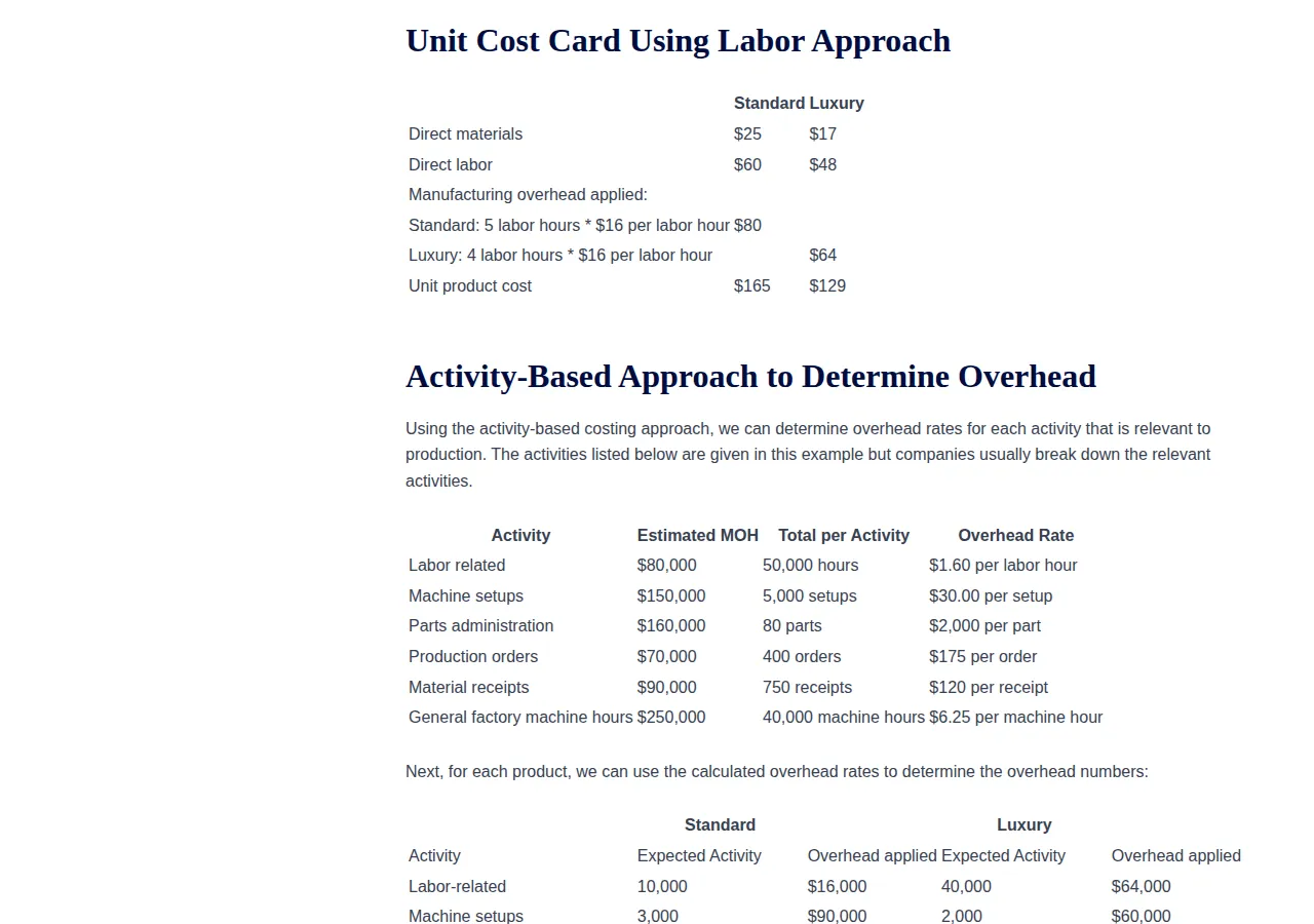
The published CFI example tells the same story with real classroom numbers. CFI's plant carries $800,000 of overhead across 50,000 labor hours, a plantwide rate of $16 per labor hour. Under that rate the Standard product costs $165 per unit and the Luxury product costs $129. Under ABC, with six activity pools, Standard costs $243.25 per unit and Luxury costs $113.35. The distortion runs the same way as in our example. Before locking a price, run the result through our profit calculator with the ABC unit cost, not the plantwide one, so the margin you see is the margin you keep.
When actual overhead misses the estimate
A predetermined rate guarantees a gap. Actual overhead is almost never the estimate, so at period end the books hold either under-applied overhead (actual above applied) or over-applied overhead (applied above actual). The gap must be cleared; it cannot sit in the overhead account into the next year.
Take actual overhead of $512,000 against applied overhead of $480,000. The shortfall is $512,000 minus $480,000, which is $32,000 under-applied. Two treatments are accepted, and the choice turns on size. When the amount is small next to the balances it touches, the whole $32,000 is charged to cost of goods sold in one entry. When the amount is large enough to distort margins, it is prorated across the accounts that hold applied overhead, in proportion to their balances. In our example the ending balances hold $48,000 of applied overhead in work in process, $144,000 in finished goods, and $288,000 in cost of goods sold, which sum to $480,000. The shares are 10 percent, 30 percent, and 60 percent. The proration is $3,200 to work in process, $9,600 to finished goods, and $19,200 to cost of goods sold, which sum to $32,000. Over-applied overhead is the mirror image, cleared the same way. A gap that repeats is an estimate that needs rebuilding from fresh factory records.
The normal-capacity rule
ASC 330 adds a guardrail that the rate alone does not provide: fixed overhead is allocated on normal capacity, not on whatever the factory happened to run. Suppose fixed overhead is $240,000 and normal capacity is 24,000 machine hours, so the rate is $10 per machine hour. If the factory runs only 20,000 hours in a slow quarter, it applies 20,000 times $10, which is $200,000, and the $40,000 that was not absorbed is expensed at once as a period charge. It is not loaded onto the fewer units produced.
Section 263A: the tax side
The reporting rule has a tax twin. Section 263A, the uniform capitalization rules, requires that direct costs and the proper share of indirect costs be included in inventory costs for property produced by the taxpayer or acquired for resale, rather than deducted at once. The statute's words in subsection (a)(2) cover the direct costs of the property and the property's proper share of indirect costs, including taxes, that are allocable to it. IRS Publication 538 carries the same rules into the accounting-methods guidance, in its Uniform Capitalization Rules section, and Publication 535, the former Business Expenses guide, was discontinued after its 2022 revision, with its topics mapped to other IRS resources.
An illustration built from the statute's categories makes the split concrete. A maker with direct materials of $120,000, direct labor of $90,000, and allocable indirect costs of $60,000 — factory rent, factory utilities, and factory equipment depreciation — capitalizes $270,000 into inventory. Selling expenses of $25,000 and general and administrative costs of $40,000, a total of $65,000, are period costs and are expensed when incurred.
The rule binds every form the business takes. A single-member LLC, an S-Corp, and a C-Corp all file under an EIN, and each one capitalizes the same way. GAAP demands absorption costing in the financial statements, and a CPA who reviews the books will test the allocation base before signing off. Even a B2B parts maker selling one SKU at a time cannot escape the rule by being small: the statute turns on producing or reselling property, not on headcount. The question is never whether the rule applies, only whether the shop's records — a CSV export of the rate sheet — can show the split under GAAP.
Month-end absorption checklist
Run this sequence every month so the year-end gap never arrives as a surprise:
- Pull actual overhead from the ledger and compare it with applied overhead for the month, so the under- or over-applied balance is visible while it is still small.
- Check the base actually used against the base budgeted, and note the variance with a one-line reason.
- Confirm every cost in the pool is a factory cost, and move any selling or office cost back to period expense.
- Recompute the rate if the factory changed — a new machine, a lost shift, a rent rise — and date the change.
- Apply overhead to jobs in progress at the current rate before closing work in process.
- Review the under- or over-applied balance and decide now whether it will be written off or prorated at year end.
- File the month's rate sheet with the estimate, the base, and the actuals.
Mistakes that misstate product cost
The most expensive mistake is the quiet one: a single plantwide rate in a factory where products use the floor in very different ways. The second is a stale rate — a base set years ago for a factory that has since automated half its lines. The third is a pool that leaks: office costs drifting into factory overhead, or abnormal waste absorbed into good units. The fourth is ignoring the under-applied balance until December, when the only fix left is a large adjustment to cost of goods sold.
Founder & CEO Insight — Enow A. Jovial
Cost allocation is not paperwork for its own sake. It is the step that turns factory spending into product truth: a rate built from real estimates, a base that tracks the work, a check against ABC when the mix is uneven, and a clean close of the gap at period end.